Neural Networks are in the center of modern Artificial Intelligence. They are responsible for most of the recent advances in AI, from machine translation to computers drawing pictures that are being sold in art auctions. In this post, we will try to understand how neural networks work.
Machine Learning
First of all, neural networks are part of broader area called Machine Learning. The main idea of machine learning is that computers can learn to do certain tasks by observing how they have been previously done by humans. Thus, we need data to train neural networks. For example, to make a neural network distinguish between a cat and a god from a picture, we need quite a lot of pictures to train it on.
| A part of Artificial Intelligence that is based on computer learning to solve the problem based on some data is called Machine Learning. To learn mode about Machine Learning, visit our Machine Learning for Beginners Curriculum. |  |
Neurons: In our Brains and in Computers
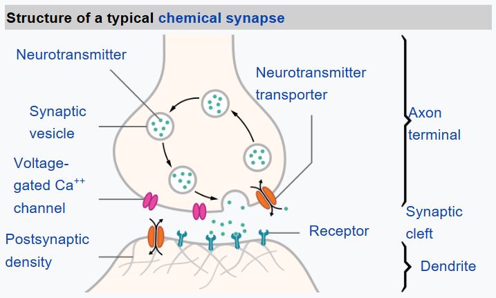
From biology we know that our brain consists of neural cells, each of them having multiple “inputs” (axons), and an output (dendrite). Axons and dendrites can conduct electrical signals, and connections between axons and dendrites can exhibit different degrees of conductivity (controlled by neuromediators).
| Real Neuron | Artificial Neuron |
|---|
 |  |
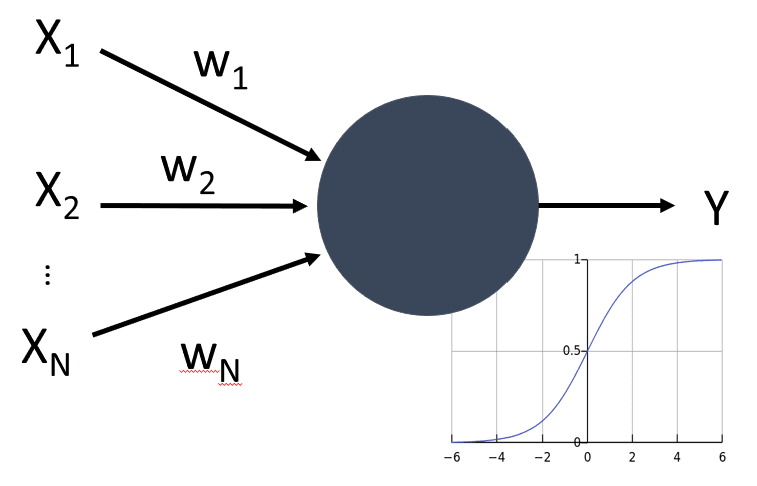
Thus, simplest mathematical model of a neuron contains several inputs $x_1,\dots,x_N$ and an output $y$, and a series of weights $w_1,\dots, w_N$. An output is calculated as
\begin{equation} y = f\left(\sum\limits_{i=1}^N x_iw_i\right)+b \end{equation}
where $f$ is some activation function, and $b$ is some number called bias.
If we represent weights as a vector $W=(w_1,\dots,w_N)$, and also take input $X=(x_1,\dots,x_N)^T$ in a vector form, our equation can be written as $y=WX+b$ (where $\cdot^T$ means transposition).
Neurons and Tensors
Suppose we want to train neural network to recognize handwritten digits, i.e. classify input image (say, or the size $28\times28$ pixels) into 10 different categories. There is a dataset called MNIST that provides around 60000 labeled images of digits that we can use to train our network.
In this case, the simplest network to do the job would have $28\times28=784$ inputs, and 10 outputs - one per class. Essentially, it will contain 10 neurons, each of them being responsible for each separate digit. Each neuron would have 784 weights and one bias value. For simplicity, we usually represent all weights in a form of a $784\times10$ matrix, where each neuron is represented by a row. Thus, the equation for our neural network can be written in a simple matrix form: $y=Wx+b$, where $W$ is weight matrix, $b$ is a bias vector, and $y$ is the network output.
When training neural networks, sometimes we need to deal with matrices of higher dimensions, which are called tensors. For example, we often take a number of training samples called minibatch. A minibatch of 100 images of size $28\times28$ can be represented by a tensor of size $100\times28\times28$.
Neural Frameworks
Modern neural networks contain millions of neurons, arranged into many layers. To train them, we need to perform a lot of matrix operations. To speed up this process, it is convenient to use GPUs, because all those computations are essentially parallel. Indeed, neurons in each layer are pretty independent.
To simplify dealing with computations on both CPU and GPU, there is a number of special framework to operate with tensors. The most popular ones are PyTorch and Tensorflow.
 |  |
| One of the first deep learning frameworks, and thus it is currently widely used in the industry. It also includes simplified Keras framework, which makes training neural networks much easier. | Great deep learning framework that is quickly gaining popularity. It first introduced the notion of dynamic computational graph, and gained huge momentum since then. |
Operating on tensors in both frameworks is pretty straightforward:
| PyTorch | Tensorflow |
data = [[1, 2],[3, 4]]
x = torch.tensor(data)
rand = torch.rand((2,2,))
ones = torch.ones((2,2,))
zeros = torch.zeros((2,2,))
res = rand+ones*x
|
x = tf.constant([[1,2],[3,4]])
rand = tf.random.normal((2,2,))
ones = tf.ones((2,2,))
zeros = tf.zeros((2,2,))
res = rand+ones*x
|
| Learn more | Learn more |
All arithmetical operations are performed element-wise. For matrix multiplication, we need to use separate operation. Dimensions are also expanded as needed.
Defining a Network
When working with neural networks in PyTorch or Tensorflow, we rarely operate on tensors directly. Rather, we define neural networks as composition of layers, where each layer contains all required parameter tensors inside it, and also defined the logic for computing and training the layer.
For example, the simplest network to recognize handwritten digits can be defined in the following way:
| PyTorch | Tensorflow/Keras |
model = Sequential(
    Flatten(),
    Linear(784,10),
    Softmax())
|
model = Sequential([
  Flatten(input_shape=(28,28)),
  Dense(10,activation='softmax')
])
|
| Learn more | Learn more |
Training a Network
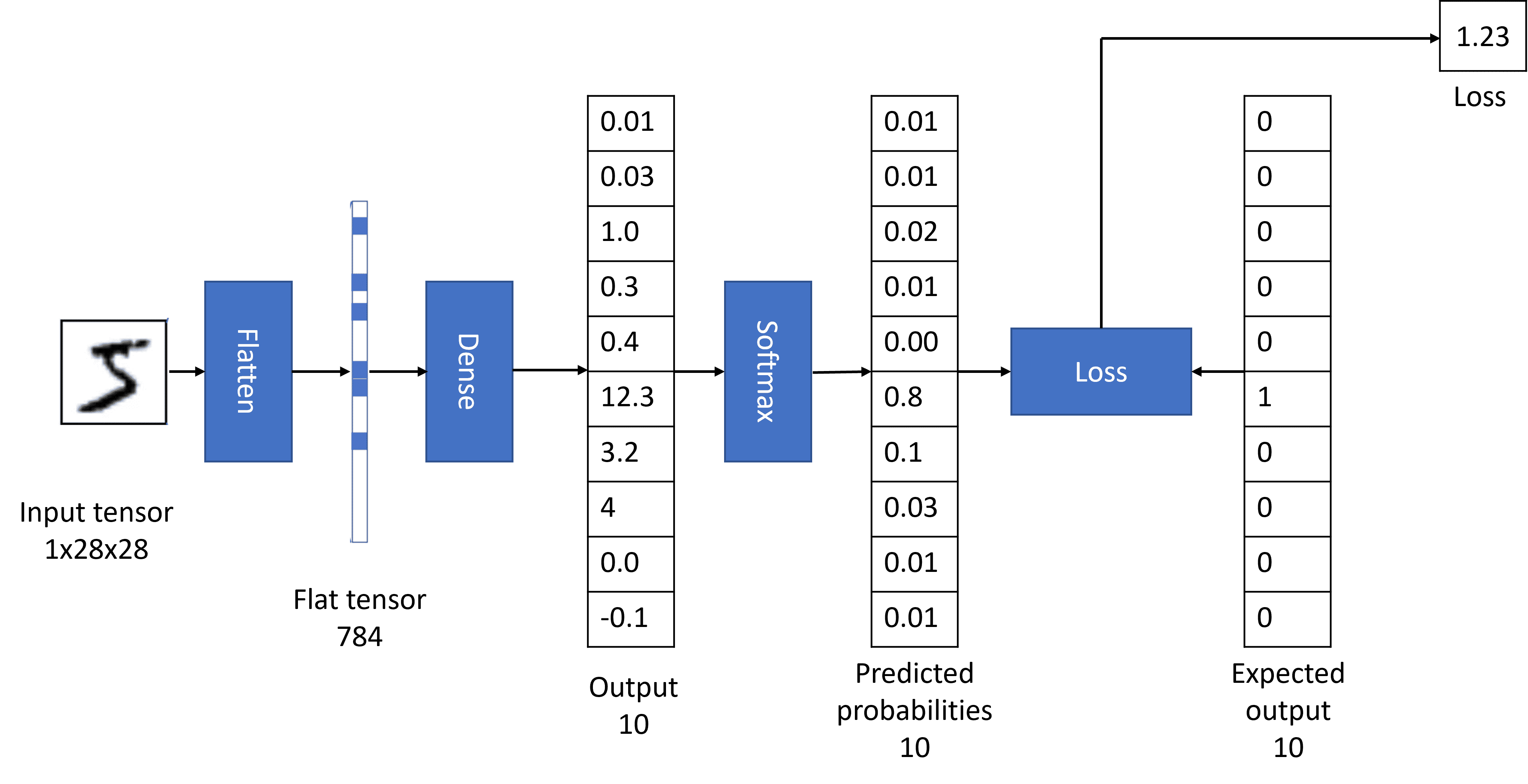
As we have discussed earlier, a network for digit recognition get an image as input, and computes the output using the formula $y=Wx+b$. The behaviour of the network is defined by its parameters: $W$ and $b$. Adjusting those parameters using training data is called training the network.
However, before we start training, there are a few things we need to add. We normally want an output of the network to represent probability, i.e. each of 10 outputs would represent a probability of the input digit representing corresponding digit. To make probabilities out of unconstrained network output we apply an activation function called softmax.

Suppose, we give our network a digit 5. Before training, we are likely to get the output that gives similar low probabilities to each of the digits. However, we want the output of our network to be $(0,0,0,0,0,1,0,0,0,0)$ — a vector that represents number 5 (this encoding is called one-hot encoding). We can calculate an error of our network using so-called loss function. As a result, we end up having a number that tells us how bad we did.
Now, to train the network, we want to adjust our parameters to minimize this error. To do it, we use mathematical procedure called gradient descent. Gradient of a function shows the direction of parameters at which the function decreases most rapidly - thus we need to compute the gradient and adjust the parameters accordingly.
All neural network frameworks allow us to compute gradients automatically. If you want, you can learn more on how this is done in PyTorch or in Tensorflow.
Before training, we need to convert our data into tensor form. If you are training on your own images, this involved loading data from disk. Usually all frameworks contain some useful functions to do that:
| PyTorch | Tensorflow |
transform = Compose([Resize(255),
                     CenterCrop(224),
                     ToTensor()])
dataset = ImageFolder('path',
                transform=transform)
dataloader = DataLoader(dataset,
        batch_size=32, shuffle=True)
|
dataset =
   image_dateset_from_directory(
     'path', batch_size=32,
    shuffle=True)
|
Some standard datasets, such as MNIST, can be loaded in more simple way, because they are built into the frameworks directly for easier access. For example, to load our handwritten digits, we need the following code:
| PyTorch | Tensorflow/Keras |
dataset = MNIST(
    root="data",
    train=True,
    download=True,
    transform=ToTensor())
dataloader = DataLoader(
    dataset, batch_size=64,
    shuffle=True)
|
(x_train, y_train), (x_test, y_test) =
       keras.datasets.mnist.load_data()
|
| Learn more | Learn more |
Training the network is done using the following algorithm:
- Repeat training several times, going through whole dataset. Each pass through the dataset is called an epoch
- Loop through the whole dataset in minibatches. At each step, we get training tensors with
images and labels. - Compute output of the network
out = net(images) - Compute the loss function
l = loss(out,labels) - Use the gradient of
l to adjust the parameters of a neural network. Typically, there is a class called optimizer that handles all the details. This process is called back propagation, because the error propagates backward through the network, adjusting all weights as it goes. - After training for an epoch, optionally compute the accuracy of the model on test dataset and store it in a list so that we can plot the training process.
In Tensorflow/Keras, this process is encapsulated inside one fit function that handles all the details. In PyTorch, you may need to describe training more verbosely:
| PyTorch | Tensorflow/Keras |
loss_fn = CrossEntropyLoss()
optimizer = SGD(model.parameters(),
            lr=0.01)
for epoch in range(10):
  for i, (X, y) in enumerate(dataloader):
    # Compute prediction and loss
    out = model(X)
    loss = loss_fn(out, y)
    # Backpropagation
    optimizer.zero_grad()
    loss.backward()
    optimizer.step()
|
model.compile(
 optimizer='sgd',
 loss='categorical_crossentropy',
 metrics=['accuracy'])

history = model.fit(x_train,y_train
 validation_data=(x_test,y_text))
|
| Learn more | Learn more |
Once we finish the training, we can use our network to make predictions by simply calling out = model(inp), where inp is the tensor with input data.
We can process several images at a time. For example, if we want to classify 20 different digits, we load their images into the tensor of size $20\times28\times28$. In this case, out tensor would have size 20\times10, and each row would give probabilities for individual input digit. To get the actual prediction, we can compute the column number with highest probability using argmax function.
Summary
This was a very short introduction to the topic of neural networks, which should nevertheless give you enough background to understand and use the code in PyTorch or Tensorflow/Keras. You can see the complete training code as one file in Pytorch. The same content as in this article is presented in more detail in Microsoft Learn modules:
Once you understand the basics, you can proceed with more specific modules on Computer Vision (PyTorch,Tensorflow), Natural Language Processing (PyTorch,Tensorflow) and more!
Happy learning!