Convolutional Neural Networks work great for image classification. There are many pre-trained networks, such as VGG-16 and ResNet, trained on ImageNet dataset, that can classify an image into one of 1000 classes. The way they work is to learn patterns that are typical for different object classes, and then look through the image to recognize those classes and take the decision. It is similar to a human being, who is scanning a picture with his/her eyes, looking for familiar objects.
 | AI for Beginners Curriculum
If you want to learn more about convolutional neural networks, and about neural networks in general - we recommend you to visit our AI for Beginners Curriculum. It is a collection of learning materials organized into 24 lessons, which can be used by students/developers to learn about AI, and by teachers, who might find useful materials to include in their classes. This blog post is based on a material from the curriculum. |
So, once trained, a neural network contains different patterns inside it’s brain, including notions of ideal cat (as well as ideal dog, ideal zebra, etc.). However, it is not very easy to visualize those images, because patterns are spread all over the network weights, and also organized in a hierarchical structure. Our goal would be to visualize the image of an ideal cat that a neural network has inside its brain.
Classifying Images
Classifying images using pre-trained neural network is simple. Using Keras, we can load pre-trained model with one line of code:
model = keras.applications.VGG16(weights='imagenet',include_top=True)
For each input image of size $224\times224\times3$, the network will give us 1000-dimensional vector of probabilities, each coordinate of this vector corresponding to different ImageNet class. If we run the network on the noise image, we will get the following result:
x = tf.Variable(tf.random.normal((1,224,224,3)))
plot_result(x)
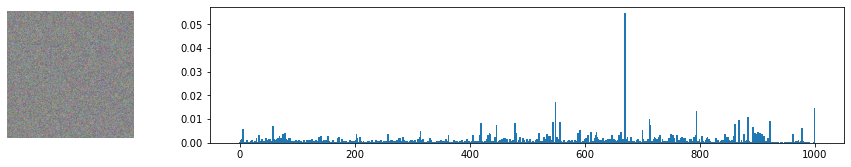
You can see that there is one class with higher probability than the others. In fact, this class is mosquito net, with probability of around 0.06. Indeed, random noise looks similar to a mosquito net, but still the network is very unsure, and gives many other options!
Optimizing for a Cat
Our main idea would be to use gradient descent optimization technique to adjust our original noisy image in such a way that the network starts thinking it’s a cat.
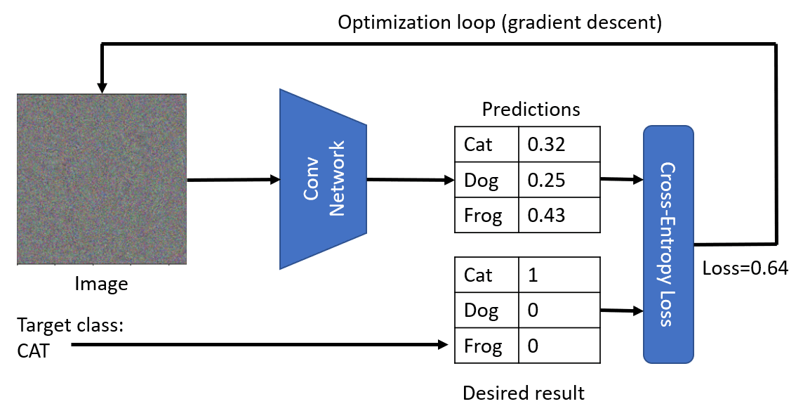
Suppose that we start with original noise image $x^{(0)}$. VGG network $V$ gives us some probability distribution $V(x^{(0)})$. To compare it to the desired distribution of a cat, we can use cross-entropy loss function, and calculate the loss $\mathcal{L} = \mathcal{L}(c,V(x^{(0)}))$.
To minimize the loss, we need to adjust our input image. We can use the same idea of gradient descent that is used for optimization of neural networks. Namely, at each iteration, we need to adjust the input image $x$ according to the formula:
\begin{equation} x^{(i+1)} = x^{(i)} - \eta{\partial \mathcal{L}\over\partial x} \end{equation}
Here $\eta$ is the learning rate, which defines how radical our changes to the image will be.
The following function will do the trick:
target = [284] # Siamese cat
def cross_entropy_loss(target,res):
return tf.reduce_mean(
keras.metrics.sparse_categorical_crossentropy(target,res))
def optimize(x,target,loss_fn, epochs=1000, eta=1.0):
for i in range(epochs):
with tf.GradientTape() as t:
res = model(x)
loss = loss_fn(target,res)
grads = t.gradient(loss,x)
x.assign_sub(eta*grads)
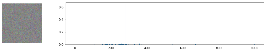
optimize(x,target,cross_entropy_loss)

As you can see, we got something very similar to a random noise. This is because there are many ways to make network think the input image is a cat, including some that do not make sense visually. While those images contain a lot of patterns typical for a cat, there is nothing to constrain them to be visually distinctive. However, if we try to pass this ideal noisy cat to VGG network, it will tell us that the noise is actually a cat with quite high probability (above 0.6):
Adversarial Attacks
This approach can be used to perform so-called adversarial attacks on a neural network. In adversarial attack, our goal is to modify an image a little bit to fool a neural network, for example, make a dog look like a cat. A classical adversarial example from this paper by Ian Goodfellow looks like this:
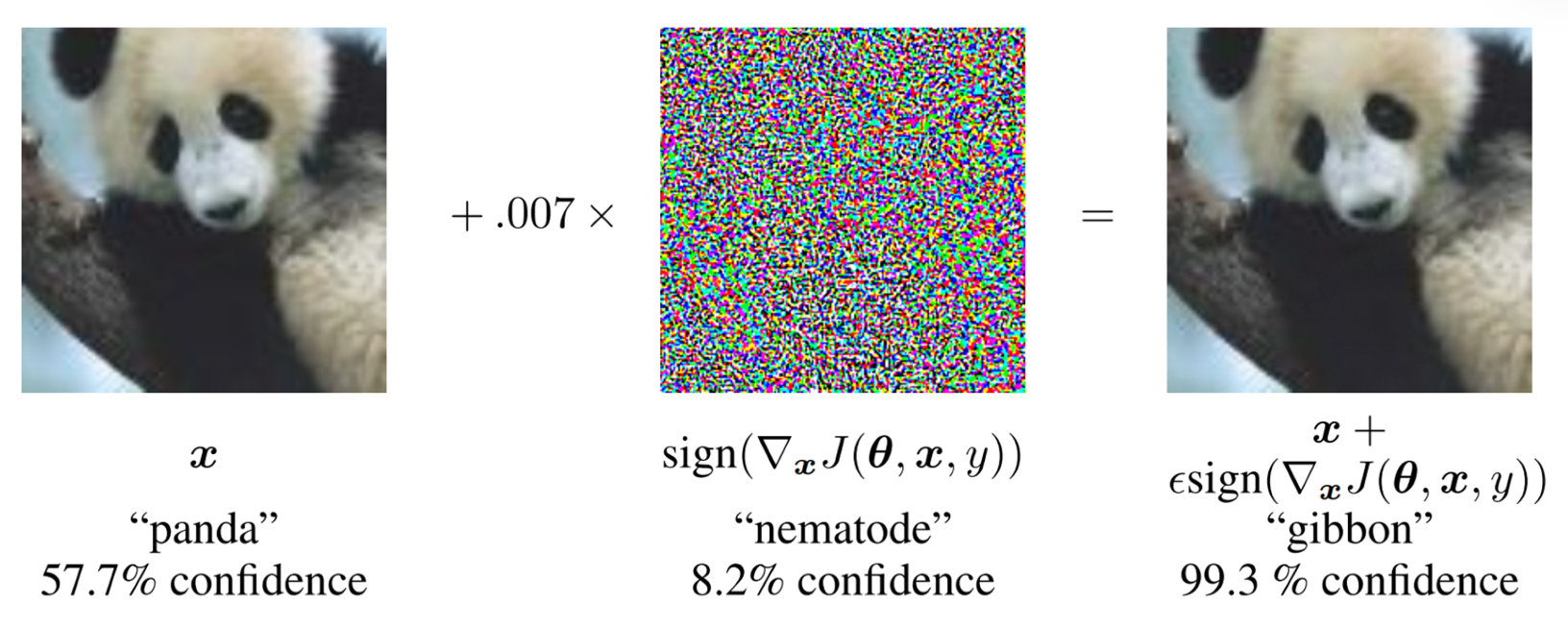
Image from the paper Goodfellow, I.J.; Shlens, J.; Szegedy, C. Explaining and harnessing adversarial examples. arXiv 2014, arXiv:1412.6572
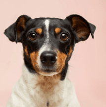
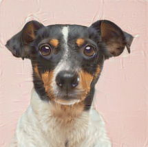
In our example, we will take slightly different route, and instead of adding some noise, we will start with an image of a dog (which is indeed recognized by a network as a dog), and then tweak it a little but using the same optimization procedure as above, until the network starts classifying it as a cat:
img = Image.open('images/dog.jpg').resize((224,224))
x = tf.Variable(np.array(img))
optimize(x,target,cross_entropy_loss)
Below you can see the original picture (classified as Italian Greyhound with probability of 0.93), and the same picture after optimization (classified as Siamese cat with probability of 0.87).
 |  |
|---|
| Original picture of a dog | Picture of a dog classified as a cat |
Making Sense of Noise
While adversarial attacks are interesting in their own right, we have not yet been able to visualize the notion of ideal cat that a neural network has. The reason the ideal cat we have obtained looks like a noise is that we have not put any constraints on our image $x$ that is being optimized. For example, we may want to constraint the optimization process so that the image $x$ is less noisy, which will make some visible patterns more noticeable.
In order to do this, we can add another term into the loss function. A good idea would be to use so-called variation loss, a function that shows how similar neighboring pixels of the image are. For an image $I$, it is defined as
\begin{equation} \mathrm{VarLoss}(I) = \sum_i\sum_j |I_{i-1,j}-I_{i+1,j}| + |I_{i,j-1}-I_{i,j+1}| \end{equation}
TensorFlow has a built-in function tf.image.total_variation that computes total variation of a given tensor. Using it, we can define out total loss function in the following way:
def total_loss(target,res):
  return 0.005*tf.image.total_variation(x,res) +\
    10*tf.reduce_mean(sparse_categorical_crossentropy(target,res))
Note the coefficients 0.005 and 10 - those are determined by trial-and-error to find a good balance between smoothness and detail in the image. You may want to play a bit with those to find a better combination.
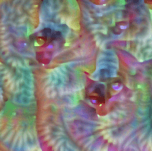
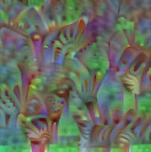
Minimizing variation loss makes the image smoother, and gets rid of noise - thus revealing more visually appealing patterns. Here is an example of such “ideal” images, that are classified as cat and as zebra with high probability:
optimize(x,[284],loss_fn=total_loss) # cat
optimize(x,[340],loss_fn=total_loss) # zebra
 |  |
|---|
| Ideal Cat, probability=0.92 | Ideal Zebra, probability=0.89 |
Takeaway
Those images can give us some insights into how neural networks make sense of images. In the “cat” image, you can see some of the elements that resemble cat’s eyes, and some of them resembling ears. However, there are many of them, and they are spread all over the image. Recall that a neural network in its essence calculates weighted sum of it’s inputs, and when it sees a lot of elements that are typical for a cat - it becomes more convinced that it is in fact a cat. That’s why many eyes on one picture gives us higher probability than just one, even though it looks less “cat-like” to a human being.
Play with the Code
Adversarial attacks and visualization of “ideal cat” are described in transfer learning section of AI for Beginners Curriculum. The actual code I have covered in this blog post is available here.