This post presents the joint research we did with Tatyana Petrova from Lomonosov Moscow State University. The code that we describe here is available on GitHub, and you can easily run it in Azure Codespaces or Azure Notebooks to do your own studies. Corresponding paper is available on preprints.org - please cite it if you use any part of the code.

Epidemic Modeling
Let’s start with the basics of how any epidemic evolves. The simples model for describing an epidemic is called SIR model, because it contains three variables:
- $S(t)$ - Susceptible - number of people who have the potential to be infected
- $I(t)$ - Infected - number of infected people
- $R(t)$ - Recovered - number of people who are non susceptible to infection (this includes the number of deceased people as well).
In this model, each variable is a function of time, and we can formulate the following differential equations that describe the behaviour of the model:
\begin{equation} \begin{array}{ll} \frac{dS}{dt} & = -\frac{βSI}{N} \cr \frac{dI}{dt} & = \frac{βSI}{N}−γI \cr \frac{dR}{dt} & =γI \end{array} \label{maineq} \end{equation}
This model depends on two parameters:
- β is the contact rate, and we assume that in a unit time each infected individual will come into contact with βN people. From those people, the proportion of susceptible people is S/N, thus the speed at which new infections occur is defined as $-\frac{βSI}{N}$.
- γ is the recovery rate, and the number 1/γ defines the number of days during which a person stays infected. Thus the term γI defines the speed, at which infected individuals are moved from being infected to recovered.
To model the epidemic, we need to solve those differential equations numerically with some initial conditions $S(0)$, $I(0)$ and $R(0)$. We will use the example from this chapter of the book [SciPyBook].
First, let’s define the right-hand-side of the differential equations:
def deriv(y, t, N, beta, gamma):
    S, I, R = y
    dSdt = -beta * S * I / N
    dIdt = beta * S * I / N - gamma * I
    dRdt = gamma * I
    return dSdt, dIdt, dRdt
Suppose we want to do the modelling for 120 days. We will define the grid of points:
days = 160
t = np.linspace(0, days, days)
Let’s model the epidemic in a large city with 12 million population – similar to the one I live in. Let’s start with 100 infected people on day 0, and assume the contact rate to be 0.2, and recovery period 30 days. Initial parameters of the model will be:
N = 12000000
I0, R0 = 100, 0
S0 = N - I0 - R0
beta, gamma = 0.2, 1./30
We will then solve the equations with the initial parameters, to obtain vectors of S, I and R for every point in our time grid:
from scipy.integrate import odeint
y0 = S0, I0, R0
ret = odeint(deriv, y0, t, args=(N, beta, gamma))
S, I, R = ret.T
plt.plot(t,S)
...
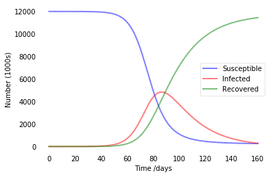
In SIR modeling, it is common to estimate the basic reproductive number of the epidemic $R_0={\beta\over\gamma}$ (see this paper for details). In our example, we were having R0=4, which is pretty similar to estimated numbers for COVID infection. So this model tells us that without any quarantine measures, in a city like Moscow we will end up with about 5 million infected people at once in about 80 days, and at the end everyone would go through the disease.
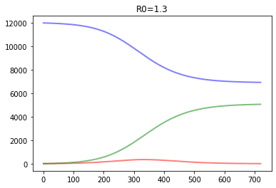
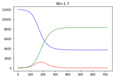
Below, we show a couple of more graphs for different R0 values:
It effectively illustrates the idea of flattening the curve, because the lower is R0 - the lower is the number of people infected at once, which helps minimize overload of healthcare system.
Determining parameters of the model
In our example, we have taken the values of β and γ somewhat freely. However, if we have some real epidemiological data, we can try to determine those values by fitting resulting SIR model to most closely correspond to real data. In this case, we will be solving optimization problem, and optimizing parameters to minimize the metric.
To get the data, we will use COVID-19 Data Repository by the Center for Systems Science and Engineering (CSSE) at Johns Hopkins University, which is available here. From this dataset, we will take the numbers of infected, recovered and deceased people, as well as the information about each country population. We will need to do some Pandas heavy lifting in order to join those tables and transpose the dates, until we get a table similar to the following for each country:
| | Date | Infected | Recovered | Deaths |
|---|
| 56 | 2020-03-18 | 147.0 | 8.0 | 0.0 |
| 57 | 2020-03-19 | 199.0 | 9.0 | 1.0 |
| 58 | 2020-03-20 | 253.0 | 9.0 | 1.0 |
| … | … | … | … | … |
We then smooth out the numbers by computing 3-days rolling average on all the columns:
for x in ['Infected','Recovered','Deaths']:
  df[x+"_Av"] = df[x].rolling(window=smooth_window).mean()
df['Removed_Av'] = df['Recovered_Av']+df['Deaths_Av']
We also compute the Removed column that contains the number of people removed from susceptible population.
We will call the resulting table country dataframe, and our code contains function make_frame, that retrieves this dataframe and population for a country given its name.
Now, to estimate R0, we need to start from a common point for all countries, let’s say, from a day when the number of infected people exceeded 1000. We will then focus on a period of several days, denoted by ndays. Taking one week into consideration seems like a good idea.
start_index = df[df['Infected_Av']>1000].index[0]
ndays = 7
V = df['Infected_Av'][start_index:start_index+ndays].to_numpy()
R = df['Removed_Av'][start_index:start_index+ndays].to_numpy()
In arrays V and R we keep the number of infected and removed people for ndays consecutive days. Now we need to define a function that will compute SIR model with given parameters β and γ, starting with number of infected/removed people at start_index, and return the error between predicted and actual data:
def model(V,R,N,beta,gamma):
    t = np.linspace(0,len(V),len(V))
    y0 = N-V[0]-R[0],V[0],R[0]
    S,I,R = odeint(deriv, y0, t, args=(N, beta, gamma)).T
    dV = np.diff(V)
    dI = np.diff(I+R)
    return np.linalg.norm(dV-dI)
The way we compute the error is the following. Because the most accurate number that we have is the accumulated number of total infected people at a given date (not considering removed ones), the easiest way would be to compute the number of new cases at each day, dV. In the SIR model, the number that corresponds to the total number of infected people will be represented by I+R, i.e. we add the number of people currently infected (I), and that have already undergone the disease (R). The number of daily new cases in the SIR model will be thus given by day-wise difference of I+R, denoted by dI. The error value returned will be the norm of the dV-dI vector.
To find parameters, we need to optimize model function with respect to parameters β and γ. In our experiment, we have found that 7 noisy data points do not allow us to optimize two parameters effectively, thus we fix γ parameter according to medical studies (see this report by WHO), that indicate mean recovery time of 30 days. We then use minimize method from SciKit Learn to find and return the optimal value of β:
the_gamma = 1/30
def fit(V,R,N):
    res = minimize(lambda x:model(V,R,N,x,the_gamma),
                          x0=0.5,method='powell')
    return res.x
Below you can find more formal mathematical description of the process. Suppose $t_0$ is the first day when the number of infected people is above 1000: $t_0=\min\{t | I(t)>1000\}$. Considering one country at a time, let us use the following denotations for the data that we have:
- $V(t)$ - the number of total (accumulated) infected cases at day $t$, $t>t_0$.
- $E(t)$ - number of recovered cases at day $t$
- $D(t)$ - number of fatal cases at day $t$
For each β, we will denote by $S_\beta(t)$, $I_\beta(t)$ and $R_\beta(t)$ the solutions of equation (\ref{maineq}) with the following initial values:
- $S(t_0)=N-V(t_0)-D(t_0)-E(t_0)$
- $I(t_0)=V(t_0)$
- $R(t_0)=D(t_0)+E(t_0)$
Here $N$ is the population of a country/city being considered. We consider the value of $\gamma=1/30$ to be fixed.
Next, we need to compare how predicted numbers correspond to the observations. The accumulated number of total infected people computed by the model is given by $I_\beta^+(t) = I_\beta(t)+R_\beta(t)$, and new total infected cases each day is equal to $I_\beta’(t) = I_\beta^+(t+1)-I_\beta^+(t)$.
The actual number of daily new infected cases $V’(t)=V(t+1)-V(t)$. We need to find the value $\beta^*$ that corresponds to the minimal discrepancy between $V’(t)$ and $I_\beta’(t)$ in the 7-day period (we will denote the number of days in consideration by $n=7$): \begin{equation} \DeclareMathOperator{\argmin}{argmin} \beta^* = \argmin_\beta\left\{\sum_{t=t_0}^{t_0+n}(V’(t)-I_\beta’(t))^2\right\} \label{betastar} \end{equation}
The process of finding argmin is complex optimization process, and at each step we need to solve an ODE (\ref{maineq}) numerically. We don’t have an explicit function for gradient, and thus we need to use some optimization algorithm that does not rely on gradients. In our case, Powell optimization provided a good compromise in terms of speed.
Once we know $\beta^*$, we can compute $R_0={\beta^*\over\gamma}$.
Here is the result we obtain for several countries available in our dataset:
| Country | R0 | Country | R0 |
|---|
| Spain | 8.269101 | Italy | 6.389969 |
| France | 6.331031 | Germany | 7.290338 |
| Brazil | 4.786171 | United Kingdom | 6.465374 |
| US | 8.257921 | Russia | 5.612825 |
| Sweden | 2.632905 | Norway | 2.816183 |
| Finland | 1.925157 | Denmark | 2.140022 |
| China | 8.342098 | Japan | 2.158008 |
| Korea, South | 6.108928 | India | 5.172934 |
Sliding SIR Estimation of Rt
In practice, it is interesting to see how the parameters of the model change over time, in reaction to protective measures implemented by different countries. Similar to the basic reproductive number R0 that is a characteristic of a disease, we can consider effective reproductive number Rt, which has the same meaning – number of people that a single infected person further infects – but during the pandemic, taking into account isolation measures and the proportion of nonsusceptible population.
We can follow the same approach for estimating Rt:
- Start from the point at which there are 1000 infected people (
start_index) - Move a sliding window with the width of 7 days (denoted by parameter
ndays) over the whole period till present day. - At each point, use 7 consecutive days to estimate β (and, thus, Rt) using
fit function above, by minimizing square difference between real and predicted number of new infected people.
To compute Rt, we find the optimal parameter β for each day, by organizing a sliding window over our country dataframe:
def compute_params(df,population, start_index, ndays):
  for i in range(start_index,len(df)-ndays):
      V = df['Infected_Av'][i:i+ndays].to_numpy()
      R = df['Removed_Av'][i:i+ndays].to_numpy()
      beta = fit(V,R,population)
      df.loc[i,'Beta'] = beta
      df.loc[i,'Gamma'] = the_gamma
Once we have the value of beta, we can compute Rt for each day in the country dataframe:
df['Rt'] = df['beta'] / df['gamma']
Some formal details are below. From mathematical point of view, to obtain $R_t$ for the day $t$, we need to find an optimal value of $\beta$ starting at $t$, instead of $t_0$. So our equation (\ref{betastar}) becomes: \begin{equation} \beta^*(t) = \argmin_\beta\left\{\sum_{i=t}^{t+n}(V’(i)-I_{t,\beta}’(i))^2\right\} \label{betastarx} \end{equation} Here $I_{t,\beta}’(i)$ also depends on $t$, because we need to consider solutions $S_{t,\beta}$, $I_{t,\beta}$, $R_{t,\beta}$ of equations (\ref{maineq}) starting with the point $t$, with the following starting conditions:
- $S(t)=N-V(t)-D(t)-E(t)$
- $I(t)=V(t)$
- $R(t)=D(t)+E(t)$.
Functions $I_{t,\beta}^+$ and $I_{t,\beta}’$ are defined in the same manner as above.
Once we get the value of Rt into country dataframe, we can explore the behaviour of the outbreak in the graphical form. Here is how epidemic unfolded in our home country, Russia: 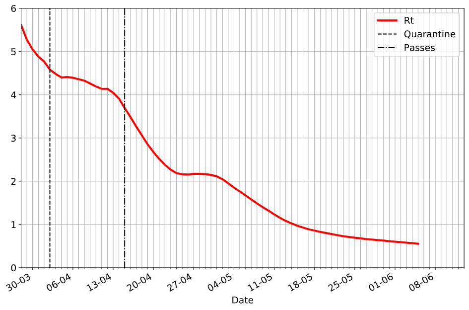
On this graph, we have indicated two dates when isolation measures were put in place:
- On April, 2nd government announced the second wave of quarantine measures (more strict than just recommended self-isolation)
- On April, 15th mandatory passes were introduced in Moscow and a few other large cities
From the graph, we can clearly see the effect of those measures on the slope of Rt curve.
To put this graph into more context, we can add the daily number of new infected cases on the same plot: 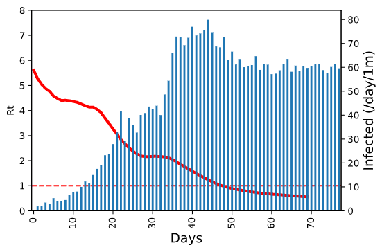 On this graph, we can also clearly see how the epidemic starts slowing down at the same time when calculated Rt value gets below 1.
To be able to compare the epidemic spread between countries, we do two things in this plot:
- on the x-axis we show the number of days since first 1000 infected cases, which makes it possible to compare the speed of the epidemic spread regardless of the actual timeframe
- the number of new cases is measured in cases per million of people, i.e. we normalize the number by country population
Comparing Epidemic in Different Countries
The data source that we are using contains the data for 188 countries, and some of them (like US) are further broken down into territories. It gives a lot of freedom to different studies and comparisons, which are not subject of this post.
However, here are the graphs from a few countries that we found interesting: 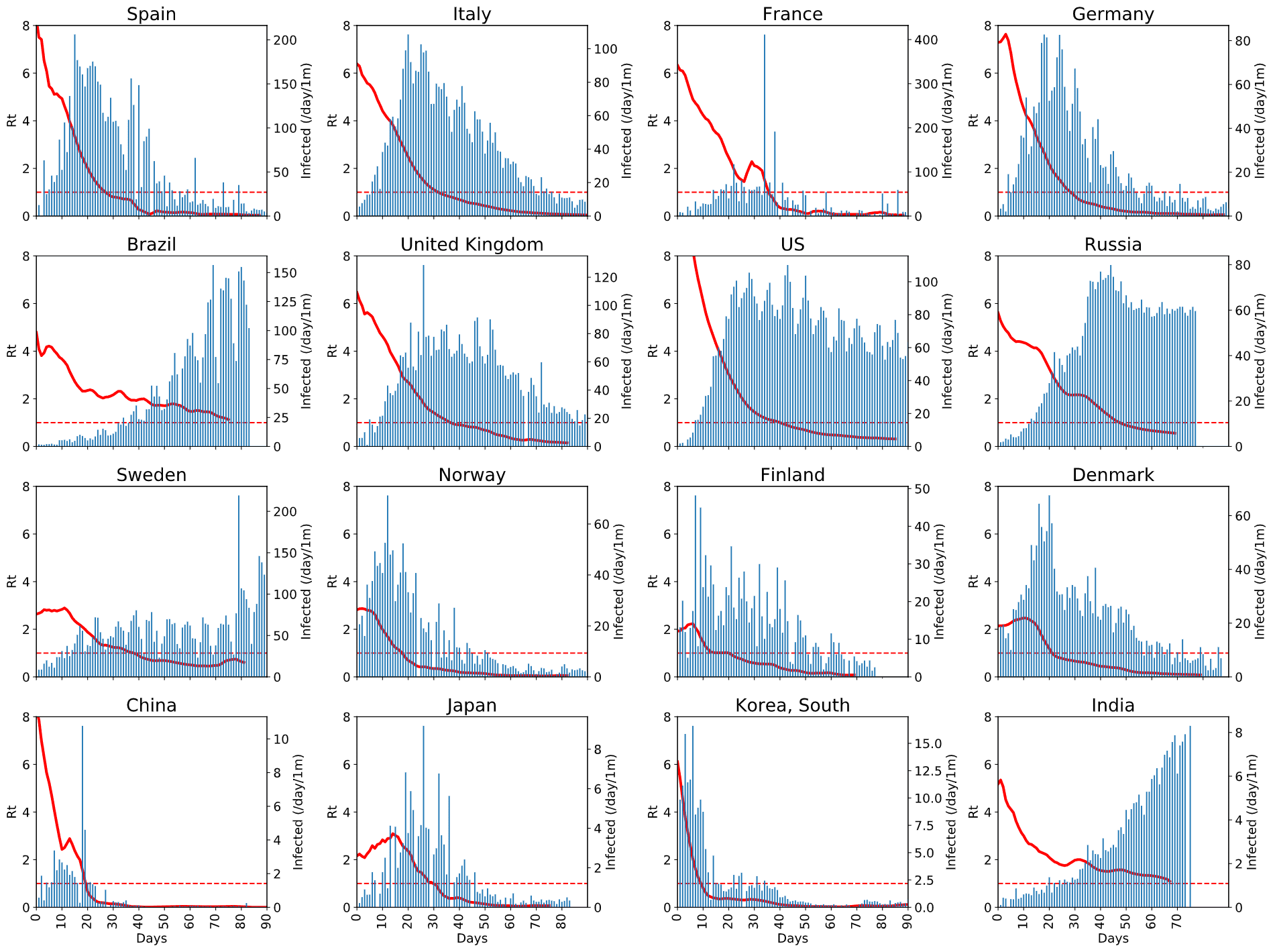 You can click on the image to enlarge it and see the details. From this graph, you can see:
- how effective protective measures in different countries are,
- how fast the epidemic is taken under control (i.e. when Rt graph gets below 1),
- how seriously it affects population overall (by the normalized number of new cases)
A few things need to be noted:
- Normalized number of new cases is shown on different scales for each graph, so you cannot compare them directly. This is done on purpose, to make the shape of the graph more visible, because in our case it seems more important than the order of magnitude.
- On all graphs we show the period from 0 to 90 days, therefore for some of the countries the graph ends earlier.
- Some graphs contain big spikes of daily new cases - this corresponds to correction in statistics. Moreover, in some cases those corrections were negative, and we do not show those on the graph. Ideally, we need to find some way to take this correction into account, because they create spikes in Rt graph, which does not happen in real life (look, for example, at the graph for France around Day 30).
To see more clearly how epidemic unrolls, it makes sense to plot all Rt graphs on one plot, starting from “Day 0”: 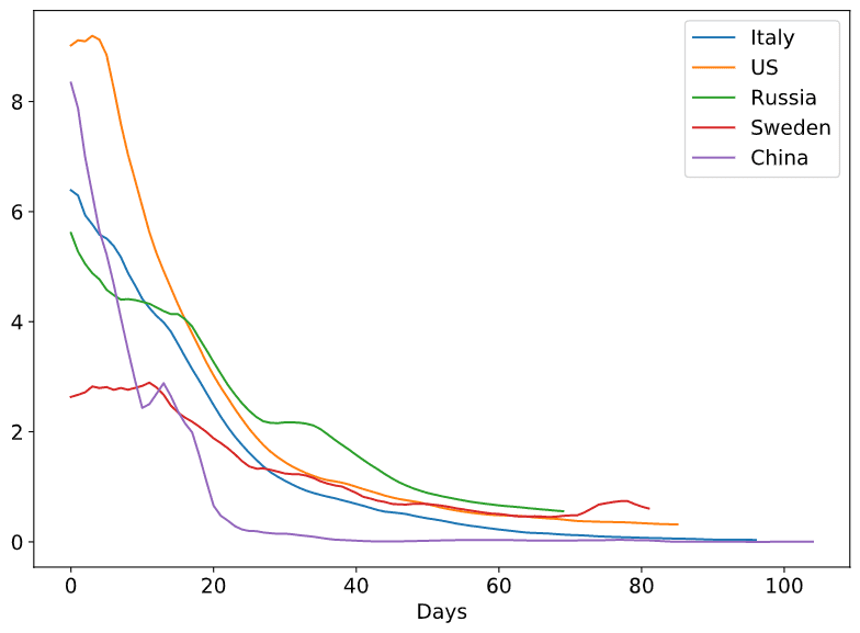
From this graphs we can clearly see how the public awareness in Sweden from the start made Rt very low comparing to other countries, but how it still less effective than quarantine measures. Also, we can see how quarantine in many countries has very similar effect on Rt, with the exception of Russia, where we can see horizontal plateau around April, 24th (possible result of permit checks in Moscow Underground on April 15th).
Here is also a plot with more countries - it looks too beautiful to be omitted, but on the other hand it is almost impossible to figure out the details. 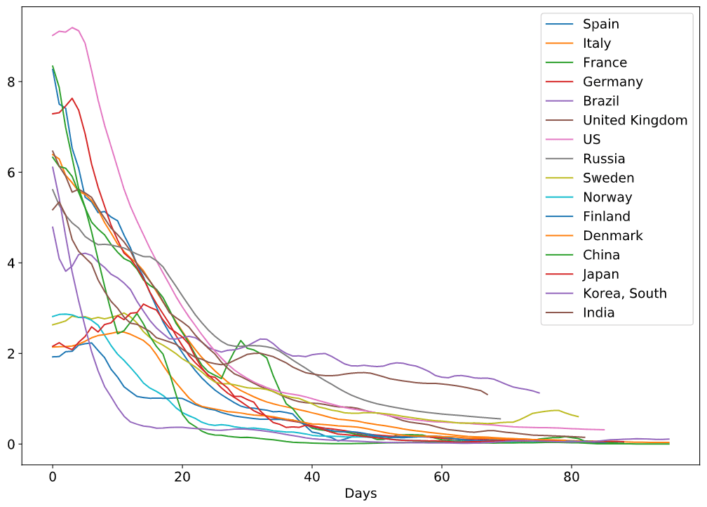
How to Cite
You are free to use the analysis code from our GitHub Repository, provided you make a link to our post, and preferably paper on preprints.org. Here is the correct reference:
Petrova, T.; Soshnikov, D.; Grunin, A. Estimation of Time-Dependent Reproduction Number for Global COVID-19 Outbreak. Preprints 2020, 2020060289 (doi: 10.20944/preprints202006.0289.v1).
The paper contains more detailed explanation of the method, a comparison with other approached to Rt estimation, and more detailed discussion of results.